What is Cost in a Query Planner?
If you ever looked at query plan from a SQL databases - you are likely to have come into something called "cost". You may even have heard that most advanced database use "cost based optimisers" But what exactly is cost and how does the database use it?
SQL Query optimisation - Introduction
The goal of a SQL query optimiser is to translate a users SQL query from "WHAT data I want to find" into a description of "HOW to find that data". This description of how to find the data is called a SQL Query Plan.
For example, the user might write this query:
SELECT C.city, SUM(S.amount)
  FROM Customer AS C
  JOIN Sales AS S
    ON S.customer_id = C.customer_id
 WHERE C.Nation = 'Estonia'
   AND S.SalesDate >= '2021-01-01'
GROUP BY C.Nation
This query does not tell us anything about HOW to retrieve the data - it simply tells us WHAT data is to be searched, joined and aggregated. This is the beauty of SQL; it moves the burden of optimising data retrieval into the database. Incidentally, this is also why NoSQL was always such a bad idea. Analysts are rarely programmers who can hand optimise queries - but they DO speak SQL. And SQL will optimise the query for them.
Optimising the query
There are many ways to execute the example query. For now, let us restrict ourselves to looking at two competing strategies
Option A
- Scan all
Customer, looking for people in Estonia. Emitcityandcustomer\_id - Build a hash table using the output of 1
- Scan
Sales, filtering out all sales that happened before 2021. Emitcustomer\_idandamount - Using the filtered sales, probe into the hash table from 2 and discard no matching customers
- Group the results
Option B
- Proceed as in option 1 step 1 and 2, building a hash table of the
Customertable on (city,customer\_id) - Scan Sales, filtering out all sales that happened before 2021. Emit
customer\_idandamount - Group the output of 1 by amount and customer_id - reducing the result in the process
- Using the reduced result in 3, probe into the hash table on
Customerto find the nation of each customer and discard the customers not in Estonia
Which one of these options is superior depends on the size/distribution of the data in the tables. But, it also depends on how expensive it is to group by or join data in the target database. If grouping is cheap, it may be faster to group BEFORE joining (option B). If grouping is expensive and joining is cheaper - option A may be superior.
Modelling Execution
Wait a minute though... what do we mean by "superior" in this case?
Typically, when we say a query plan is "superior" to another - we mean that it runs faster. Users are impatient creatures who like instant gratification. It seems like the database should attempt to predict the runtime of the query and pick the query plan that has the lowest, predicted runtime.
Predicting runtimes is tricky. Even when the query optimiser has perfect knowledge about the data - it still needs a model of execution. A model of execution must translate row counts, row width, data types, memory usage and many other factors into a prediction about how long the database engine will take to evaluate each part in the query. Not only that, it must also take the target hardware into account. Even if I know that I can join 40M rows / CPU core on a single core AMD - does it follow that I can join 64x times that on an AMD Epyc 64 core CPU? Does the same values hold for Intel? How about ARM? What about DRAM types and L3 cache sizes which influence join speed. Does it matter if the database engine is MySQL, Postgres, SQL Server or Yellowbrick? If the system is distributed - we also need to factor network speeds into the equation.
Correctly predicting runtime is a multi variate problem that requires very fine calibration of the query optimiser to a great many scenarios. Fortunately, it turns out that we typically don't need to take all those variables into account.
Relative Time matters
Consider again our sample query. Deciding between Option A and Option B boils down to answering this question:
"Is is faster to GROUP than to JOIN with the row counts given in this query?"
It turns out that the answer does not depend on the target hardware. Well, to a good enough approximation anyway. What we really care about is the relative runtimes of grouping vs joining. We might not be able to predict the exact time the query will run. But, we don't need to, as long as we know which one of A and B are likely to run faster. In the vast majority of cases - which one runs faster does not depend on what HW we have.
Instead of talking about the time it takes to join vs group - we instead introduce the notion of "cost". Cost is unitless - since we don't really care about its absolute value. Its only used to compare one query plan against another. Using this new term, we might express a rough model of execution in these terms:
Let W be the width of the row we operate on.
- The cost of joining one row is some constant (Cjoin), multiplied by the W, multiplied by the size of the
- hash table being joined (JR)
- The cost of grouping one row is some constant (Cgroup), multiplied by W
Obviously, for real life examples, W, JR and the Cjoin / Cgroup are not the only factors influencing the costs. But for the purpose of understanding cost, its good enough.
The problem of picking between A and B now boils down to picking representative values of Cjoin and Cgroup.
Calibrating the model
Our simplified model looks like this (per row):
Cost group = Cgroup * W
Cost join = Cjoin * W * JR
To calibrate this model, we can run a series of tests comparing grouping a joining. For example, we might pick two queries for joining and grouping like these
SELECT some_col
FROM Test
GROUP BY SomeCol

SELECT Test.some_col
FROM Test
JOIN TestJR ON test.id = TestJR.id
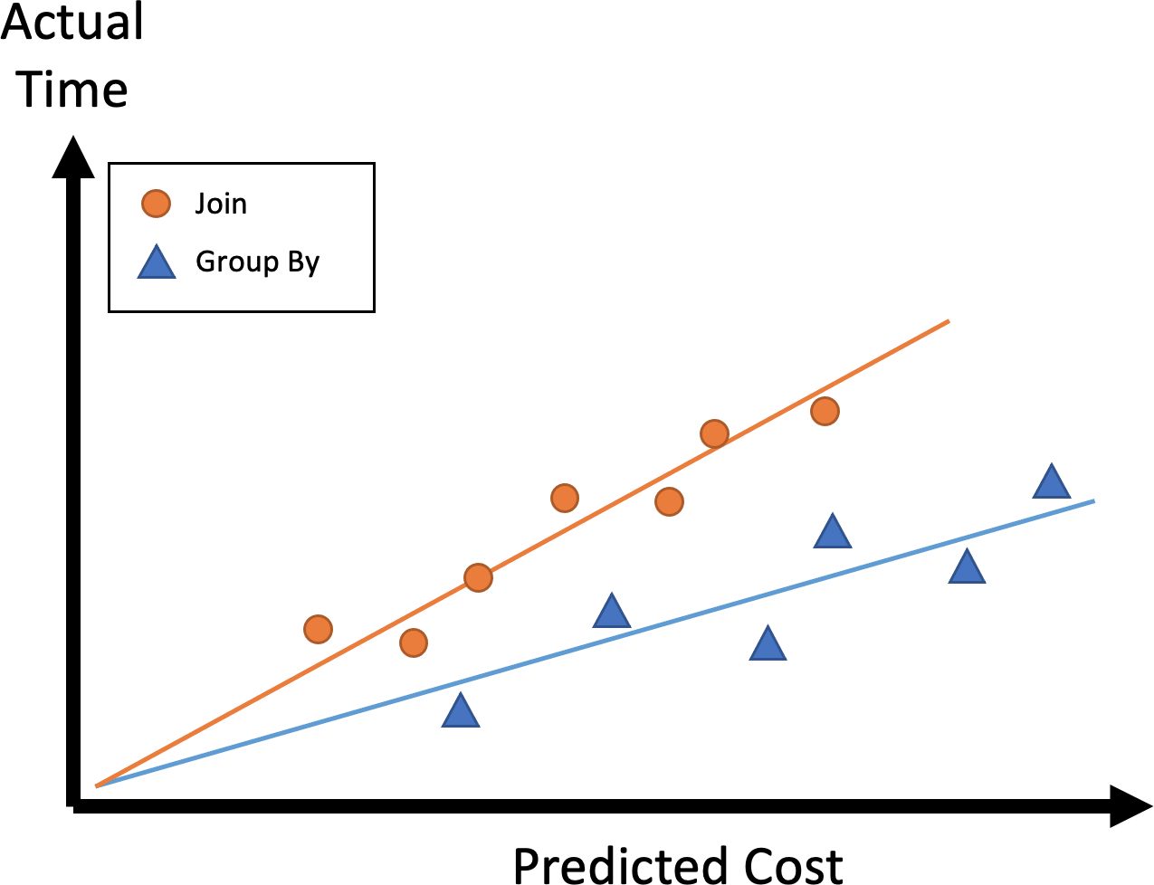
We would then vary the width of some_col (W in the model) and the number or rows in TestJR (`JR`` in the
model) and plot the actual runtime vs the cost. What we are looking for is a strong correlation between the measured
runtime and the cost predicted by the constants Cjoin / Cgroup.
Let us say that for some initial value of the constant, we get a plot like this:

First, we would be encouraged to find that our model of a linear dependency appears to be reasonably fine. Second, we can see that for the values chose for Cjoin and Cgroup are a bit off. We should probably pick a value for Cjoin that is slightly higher. Remember, we just care about the relative value of the cost constants. What we are looking for is something like this:

Notice that we are calibrating the constants using actual, measured wall clock time on some reference system. There are few different design philosophies for database engine about what to do next once we have the calibration right.
- Use the reference system calibration for all other other hardware
- Rerun cost calibration whenever the database is installed on a new hardware
- Create a feedback loop, slowly adjusting the cost constant based on measurements on the currently running system
Its not clear which one of these strategies is superior.
Ad 1) The advantage of this strategy is that cost values and the query plan choices they drive is consistent across all
HW platforms. For a DBA that is used to queries behaving in a certain, predictable, way this is often preferable -
even when upgrading hardware. The downside is of course that some hardware can in fact do certain operations
relatively faster than others. For example, the join algorithm that is optimal on AMD isn't always optimal in Intel -
which may change the GROUP BY / JOIN calibration.
Ad 2) This seems tempting if you know what HW you are going to run on and you want to get the best out of it. The downside is that once you are in a cloud - you generally have no idea what HW you end up running on. Not only that - the number of nodes making up a distribute database may change in elastic environments - so any calibration you do has the same issues as 1.
Ad 3) At first glance, this would seem like the best of both worlds. However, it is not a panacea. For example, in a batch style environment the ETL running at night may lead to a specific cost calibration of the system that does not serve reporting users in the morning well. It can also be a nightmare of the DBA to deal with query plans that suddenly change for the worse because the system decided to recalibrate costs.
Adding up the example
Using our calibrated cost model, we can now compare Option A and option B.
First, we notice that the scan costs must be the same. Both queries need to scan Sales and Customer for the same
data. Any costing model we had for scans is hence irrelevant.
Let:
|CustomerEstonia| ::= Row count of Customer after filtering out Estonia
|Sales2021| ::= Row count of sales in 2021
|Sales2021 ⨝ CustomerEstonia| ::= Row count of the join between the two above
W(city) ::= Avg Width of City Column
Option A (join before group)
Cost of the join:
|Sales2021| * (W(city) + W(amount)) * |CustomerEstonia| * Cjoin
Cost of the group after join
|Sales2021 ⨝ CustomerEstonia| * Cgroup
Option B (group after join)
Cost of the group
|Sales2021| * Cgroup
Cost of the join:
|Customer| * (W(city) + W(amount)) * |CustomerEstonia| * Cjoin
(note we can multiply by |Customer| as the grouping will reduce the input from Sales to the number of unique customers)
Depending on what cost constants we calibrated, we can now plug those into the equations and simply pick A or B depending on which has the lower cost.
Conclusion
In this blog, we have provided a brief introduction to the notion of Cost in databases. There is a lot more to be said about it - which is the subject of a future blog.
But today, what you hopefully learned is that
- Cost is a unitless quantity used to compare query plans
- The equations for calculating cost will often take many variables into account
- Cost must be calibrated for all the operations the database can do. The calibration must take the relative runtimes of the operations into account
- Costs, even for the same query, may vary across different hardware platforms - this depends on the database vendor.


 11 min


